MC Grating
Step-by-step examples
The examples document, page by page: which structure file to open, what to press, and what you should see. All structures are adapted to demo mode's limits.
The structure files for every example are in Examples-Structures.zip; the original document is Examples-Description.pdf. Sections are numbered as in the document: 1–3 the Chandezon codes, 4–6 the modal codes.
1 Chandezon collinear
1.1 Classic
1.1.1 The example of a single resonance excitation in a corrugated waveguide by a plane wave having the TE polarization under 45 degrees incidence.
Settings are arranged for the E-field modulus scanning inside the structure and in ambient media.
Open the source file Single_TE_Res_45deg.cha and press the Run button and then press the Graph button. If necessary, in the Graph window go to View and select Front.
1.1.2 The example of a double resonance excitation in a corrugated waveguide by a plane wave having the TE polarization under normal incidence.
Settings are arranged for:
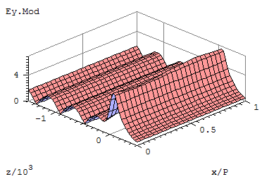
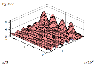
a) The E field modulus scanning inside the structure and in ambient media. Open the source file Doub_TE_Res_Refl_Field.cha and press the Run button and then press the Graph button. If necessary, in the Graph window go to View and select Front.
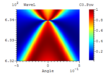
b) Reflection scanning versus angle and wavelength both close to the resonance values. Go to Settings -> Scanning and enable page Scanning. Press the Run button and wait for result and then press the Graph button. If necessary, in the Graph window go to View and select Top Color Image and Color Scale.
1.1.3 The example demonstrates high efficient metal sinusoidal grating in Littrow condition for the TE polarization. A substrate refractive index is close to the Aluminum real value refractive index at the 1000 nm wavelength.
Open the source file Littrow.cha and press the Run button for evaluating diffraction efficiencies. Press the Run button again and then press the Graph button. If necessary, in the Graph window go to View and select Top Color Image and Color Scale.
1.1.4 The example of a Littrow reflection versus incident angle of a plane wave having the TM polarization from a triangular copper grating for rear copper mirror CO2 laser of radial polarization. Advanced scanning was used with the expectation that the incident radiation was normal for a leg of the triangle. There are two variants: first - the scan data were prepared outside the MC Grating code in form of the built-in table and second – the incident conditions are provided by the built-in equations.
This example was designed to investigate of a Littrow reflection versus incident angle of a plane wave having the TM polarization from a triangular copper grating. This calculation is due to the further application of optimal parameters for the design of a concentric diffraction grating on the surface of the copper cone rear mirror for the radial polarization selection of CO2 laser.
Open the source file Littrow_CO2_Table.cha or. Littrow_CO2_Equations.cha.
a) Press the Run button and then press the Graph button, select ANG_4 as a X column and press OK button. b) To see the TE - TM reflection contrast. Go to General, change Polarization to TE and repeat the previous instructions (with red curve color).
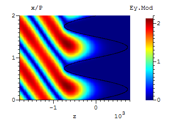
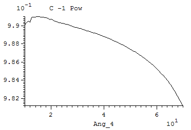
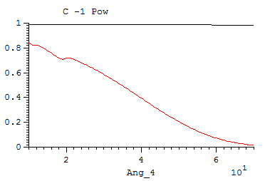
To see reflection coefficient and field distribution open the source file Littrow_CO2_Fld.cha. Press Run, then once again the key and button Graph. If necessary, in the Graph window go to View and select Top Color Image and Color Scale.
1.1.5 The example of abnormal mirror for laser diode array synchronization The example is taken from the paper Quantum Electronics 42(6) 561-564(2012) and is
adapted for demo mode.
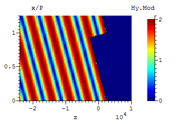
Open the source file Abnormal_Mirror.cha.
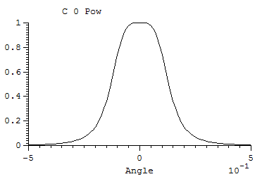
a) For evaluating angular reflection spectrum press the Run and the Graph button.
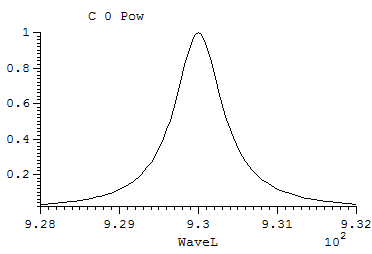
b) For evaluating wavelength reflection spectrum go to Settings -> Scanning select Wavelength as Scanning of, press the Run and the Graph button.
c) Press the Optimize button to evaluate optimization functionality.
1.2 Extended
1.2.1 The example of a double resonance excitation in a corrugated waveguide by a plane wave having the TM polarization under normal incidence.
Settings are arranged for:
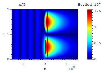
a) Magnetic field modulus scanning inside the structure and in ambient media. Open the source file Doub_TM_Res_Refl_Field.cha and press the Run button and then press the Graph button. If necessary, in the Graph window go to View and select Top Color Image and Color Scale.
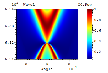
b) Reflection scanning versus angle and wavelength both close to the resonance values. Go to Settings -> Scanning and enable page Scanning. Press the Run button and wait for result then press the Graph button.
2 Chandezon conical
2.1 Classic
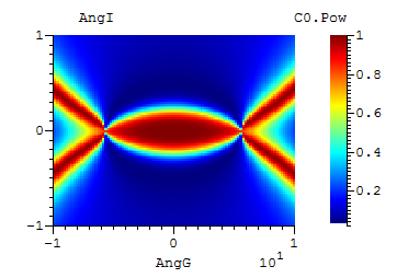
2.1.1 The example of a double resonance excitation in a corrugated waveguide by a plane wave having the TE polarization under normal incidence. The example also demonstrates the Grating based coordinate system use.
Settings are arranged for reflection scanning versus two angles close to the normal. The incidence wave E field projection on a structure plane remains parallel to the grating grooves. Open the source file Doub_TE_Res_AngI_AngG.cha and press the Run button and wait for result then press the Graph button. If necessary, in the Graph window go to View and select Top Color Image and Color Scale.
2.2 Extended
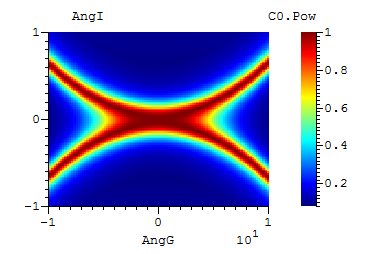
2.2.1 The example of a double resonance excitation in a corrugated waveguide by a plane wave having the TM polarization under normal incidence.
Settings are arranged for the reflection scanning versus two angles close to the normal. Incidence wave H field projection on structure plane remains parallel to the grating grooves. Open the source file Doub_TM_Res_AngI_AngG.cha and press the Run button and wait for result then press the Graph button. If necessary, in the Graph window go to View and select Top Color Image and Color Scale.
3 Chandezon crossed
3.1 Classic
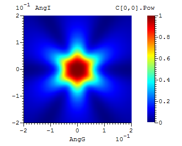
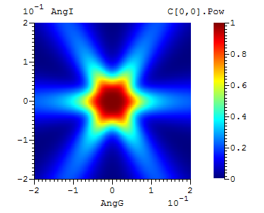
3.1.1 The example of a hexagonal grating of high period resonance excitation in all interfaces corrugated waveguide by a plane wave near normal incidence.
The example also demonstrates the Grating based coordinate system use.
a) Settings are arranged for reflection scanning versus two angles close to the normal.
The incidence wave has the TE polarization state (State angle equals to zero).
To see a TE polarization incidence open the source file Classic_High_Per.cha press the Run button and wait for several hours. Software will calculate a reflection for positive angles quarter. When calculation will be finished position mouse to result area, press the right mouse button and select Symmetrize Data option to extend results for negative angles (instead of all the previous open file Classic_High_Per_TE.dat) and press the Graph button. If necessary, in the Graph window go to View and select Top Color Image and Color Scale.
b) To see a TM polarization incidence wave reflections go to Settings -> General and change the State angle to 90 degrees, press the Run button, Symmetrize Data (instead of all the previous open file Classic_High_Per_TM.dat) and press the Graph button.
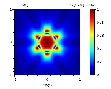
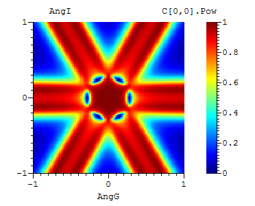
3.1.2 The example of a hexagonal grating of low period resonance excitation in all interfaces corrugated waveguide by a plane wave near normal incidence.
The example also demonstrates the Grating based coordinate system use.
a) Settings are arranged for reflection scanning versus two angles close to the normal. The incidence wave has the TE polarization state (State angle equals to zero).
To see a TE polarization incidence open the source file Classic_Low_Per.cha press the Run button and wait for several hours. Software will calculate a reflection for positive angles quarter. When calculation will be finished position mouse to result area, press the right mouse button and select Symmetrize Data option to extend results for negative angles (instead of all the previous open file Classic_Low_Per_TE.dat) and press the Graph button. If necessary, in the Graph window go to View and select Top Color Image and Color Scale.
b) To see a TM polarization incidence wave reflections go to Settings -> General and change the State angle to 90 degrees, press the Run button, Symmetrize Data (instead of all the previous open file Classic_Low_Per_TM.dat) and press the Graph button.
3.2 Extended
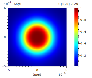
3.2.1 The extended method example of a hexagonal grating of high period resonance excitation in a cover interface corrugated waveguide by a plane wave near normal
incidence.
The example also demonstrates the Grating based coordinate system use.
a) Settings are arranged for reflection scanning versus two angles close to the normal.
The incidence wave has the TE polarization state (State angle equals to zero).
To see a TE polarization incidence open the source file Extended_High_Per.cha press the Run button and wait for several hours. Software will calculate a reflection for positive angles quarter. When calculation will be finished position mouse to result area, press the right mouse button and select Symmetrize Data option to extend results for negative angles (instead of all the previous open file Extended_High_Per_TE.dat) and press the Graph button. If necessary, in the Graph window go to View and select Top Color Image and Color Scale.
b) To see a TM polarization incidence wave reflections go to Settings -> General and change the State angle to 90 degrees, press the Run button, Symmetrize Data (instead of all the previous open file Extended_High _Per_TM.dat) and press the Graph button.
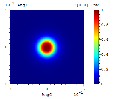
3.2.2 The extended method example of a hexagonal grating of low period resonance excitation in a cover interface corrugated waveguide by a plane wave near normal
incidence.
The example also demonstrates the Grating based coordinate system use.
a) Settings are arranged for reflection scanning versus two angles close to the normal.
The incidence wave has the TE polarization state (State angle equals to zero).
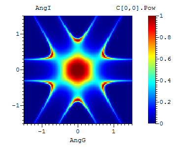
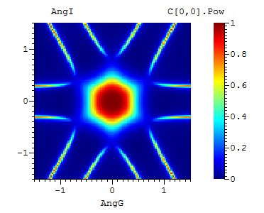
To see a TE polarization incidence open the source file Extended_Low_Per.cha press the Run button and wait for several hours. Software will calculate a reflection for positive angles quarter. When calculation will be finished position mouse to result area, press the right mouse button and select Symmetrize Data option to extend results for negative angles (instead of all the previous open file Extended_Low_Per_TE.dat) and press the Graph button. If necessary, in the Graph window go to View and select Top Color Image and Color Scale.
b) To see a TM polarization incidence wave reflections go to Settings -> General and change the State angle to 90 degrees, press the Run button, Symmetrize Data (instead of all the previous open file Extended_Low_Per_TM.dat) and press the Graph button.
4 Modal collinear
4.1 The example demonstrates the grating having zero transmission in zero
order for the TE polarization.
Open the source file ZeroTransm_0-order.mdl. There are several successive options:
a) Press the Run button to evaluate diffraction efficiencies.
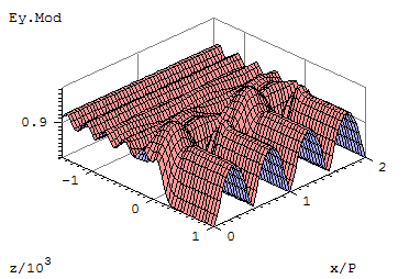
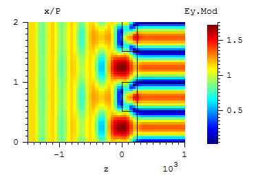
b) Press the Run button again and then press the Graph button for the field distribution. If necessary, in the Graph window go to View and select Back.
c) In the Graph window go to View and select Top Color Image and Color Scale.
d) Press the Optimize button to evaluate optimization functionality.
4.2 The example of a multilayer mirror design using an optimization.
The example is taken from the paper Quantum Electronics 30(1) 13- 14(2000) and is adapted for demo mode.
Open the source file MLMirror.mdl. There are several options: a) Press the Run button and then press the Graph button to see a Mirror wavelength reflection graph.
b) Press the Optimize button to evaluate the optimization functionality.
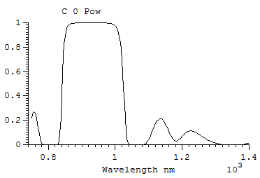
4.3 The example of modes filtering effect for high refractive index contrast
ideal metal grating. The example is taken from the paper J. Opt. Soc. Am. A, Vol. 24, pp. 3781-3788 (2007) and is adapted for demo mode.
Settings are arranged for the field calculation and for the diffraction efficiency scan versus groove width.
Open the source file RCWA.mdl. There are several successive options.
a) For the FMM field calculation with modes filtering press the Run button. When the calculation is finished press the Graph button.
b) For the FMM field calculation without modes filtering go to Setting -> Options uncheck Neff Filter Level box. Press the Run button. When the calculation is finished press the Graph button.
c) For the TMM field calculation go to Setting -> General select True Modes. Press the Run button. When the calculation is finished press the Graph button.
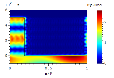
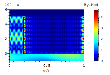
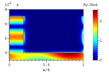
d) For the TMM diffraction efficiency scan go to Setting -> Options uncheck Field Calculation box. Press the Run button. When the calculation is finished press the Graph button. e) For the FMM diffraction efficiency scan without modes filtering go to Setting -> General select Fourier Modes. Press the Run button. When the calculation is finished press the Graph button and select red color. f) For the FMM diffraction efficiency scan with modes filtering go to Setting -> Options. check Neff Filter Level box. Press the Run button. When the calculation is finished press the Graph button and select blue color.
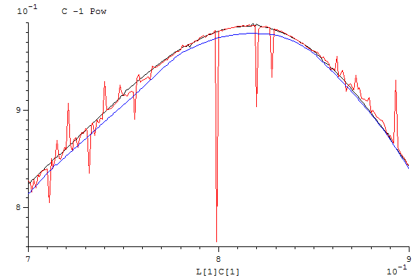
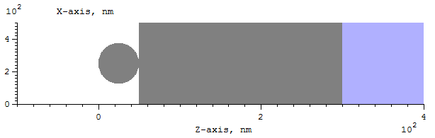
4.4 The example of a grating profile generation from a data file. Open any sample from the File -> Samples menu. Go to Settings -> Layers and press the Convert button to open Layer Conversion window. For example type 100 in the field Number of Sub Layers. In Conversion Type combo box select the Profile From File item and then from the Profile files -> Modal 1D folder select ProfileCylinder 1 data file and press OK button. Close the Settings window and go to the Service Window -> Grating Profile menu to evaluate the grating profile.
5 Modal conical
5.1 The example demonstrates the grating having zero transmission in zero order under normal incidence. The example also demonstrates the Grating
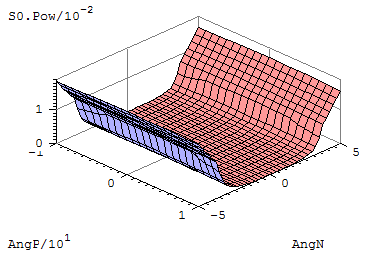
based coordinate system use. Settings are arranged for evaluating the zero order transmission versus two angles around normal preserving the vector E projection on the structure plane parallel to the grating grooves.
Open the source file ZeroTransm_AngN_AngP.mdl and press the Run button and wait for result, then press the Graph button. If necessary, in the Graph window go to View and select Front.
5.2 The example demonstrates the Slider functionality.
Open the source file Slider.mdl. Press the Run button. In a few seconds the angular reflection from a corrugated waveguide will be calculated. Press the Slider menu item and evaluate the reflection behavior versus incident wave polarization state and the output polarizer orientation.
6 Modal crossed
6.1 The modal method example of a hexagonal grating of high period resonance excitation in a cover interface corrugated waveguide by a plane
wave near normal incidence. The example also demonstrates the Grating based coordinate system use.
a) Settings are arranged for reflection scanning versus two angles close to the normal.
The incidence wave has the TE polarization state (State angle equals to zero).
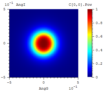
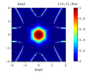
Open the source file High_Period.mdl press the Run button and wait for several hours. Software will calculate a reflection for positive angles quarter. When calculation will be finished position mouse to result area, press the right mouse button and select Symmetrize Data option to extend results for negative angles (instead of all the previous open file High_Period _TE.dat) and press the Graph button. If necessary, in the Graph window go to View and select Top Color Image and Color Scale.
b) To see a TM polarization incidence wave reflections go to Settings -> General and change the State angle to 90 degrees, press the Run button, Symmetrize Data (instead of all the previous open file High_Period _TM.dat) and press the Graph button.
6.2 The modal method example of a hexagonal grating of low period resonance excitation in a cover interface corrugated waveguide by a TE plane
wave near normal incidence. The example also demonstrates the Grating based coordinate system use.
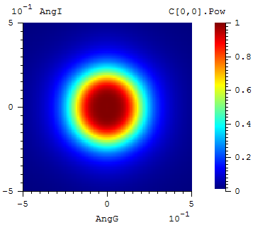
a) Settings are arranged for reflection scanning versus two angles close to the normal. The incidence wave has the TE polarization state (State angle equals to zero). Open the source file Low_Period_TE.mdl press the Run button and wait for several hours. Software will calculate a reflection for positive angles quarter. When calculation will be finished position mouse to result area, press the right mouse button and select Symmetrize Data option to extend results for negative angles (instead of all the previous open file Low_Period_TE.dat) and press the Graph button. If necessary, in the Graph window go to View and select Top Color Image and Color Scale.
6.3 The modal method example of a hexagonal grating of low period resonance excitation in a cover interface corrugated waveguide by a TM plane
wave near normal incidence. The example also demonstrates the Grating based coordinate system use.
a) Settings are arranged for reflection scanning versus two angles close to the normal. The incidence wave has the TM polarization state (State angle equals to 90 degrees)
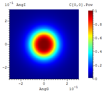
Open the source file LowPeriodTM.mdl press the Run button and wait for several hours. Software will calculate a reflection for positive angles quarter. When calculation will be finished position mouse to result area, press the right mouse button and select Symmetrize Data option to extend results for negative angles and (instead of all the previous open file Low_Period _TM.dat) press the Graph button. If necessary, in the Graph window go to View and select Top Color Image and Color Scale.
6.4 Advanced scanning and advanced output. There are two variants: first - the scan data were prepared outside the MC Grating code in form of the built- in table and second - the structure parameters are provided by the built-in
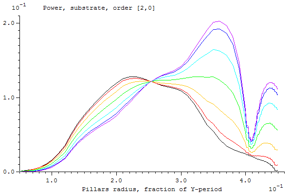
equations This example was designed to investigate hexagonal binary grating of circular pillars for diffraction efficiency versus radius of pillars as a fraction of a smallest dimension of elementary grating cell. For this purpose the purely theoretical grating model was used. Pillars of refractive index 2 is “free suspended” in media of refractive index 1. The scanning data was prepared outside the MC Grating software and has two parts: first part with radius step of 0.01 and second part around peculiarity with step of value 0.001. In the figure there are presented graph of diffraction efficiency curves for the substrate (2,0) order. Curves correspond to different polarization states of incident wave from the TE (black) to the TM (violet) with respect to the diffracted wave (angular step is 15 degrees). Diffraction orders (2,0), (1,1), (1,-1), (-1,1), (-1,-1), (-2,0) are physically equivalent owing to the grating symmetry and have the same dependence versus the polarization state of incident wave.
Open the source file Efficiency_Pilllar_Radius_Table.mdl or Efficiency_Pilllar_Radius_Equations.mdl press the Run button and wait for quarter of an hour. Software will calculate a reflection scan for the TE polarization. Draw this scan curve end goes back to Scanning -> General and increase the polarization state by 15 degrees. Press the Run button. Recalculation will take a couple of seconds. Repeat these steps up to the TM polarization (90 degrees of polarization state). After finishing scanning by source file it is also possible to analyze the polarization behavior by Slider option.
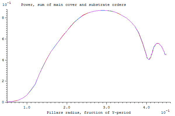
Advanced output adds an additional column for the output with a power sum of all main diffracted orders (six transmitted and six reflected). A series of seven plots, under the same conditions as a graphic in the previous figure, is set out below.
This figure allows us to conclude that the total diffraction efficiency of a hexagonal grating in the basic order does not depend on the orientation of the electric vector of the incident wave at normal incidence.